NOMAD: the oceaN frOnt dataset for the Mediterranean seA and southwest inDian ocean
Fronts are ubiquitous discrete features of the global ocean often associated with enhanced vertical velocities, in turn boosting primary production and so forth. Fronts thus form dynamical and ephemeral ecosystems where numerous species meet across all trophic levels. Fronts are also targeted by fisheries. Capturing ocean fronts and studying their long-term variability in relation with climate change is thus key for marine resource management and spatial planning. The Mediterranean Sea and the Southwest Indian Ocean are natural laboratories to study front-marine life interactions due to their energetic flow at sub-to-mesoscales, high biodiversity (including endemic and endangered species) and numerous conservation initiatives. Based on remotely-sensed Sea Surface Temperature and Height, we compute thermal fronts (2003-2020) and attracting Lagrangian Coherent Structures (1994-2020), in both regions over several decades. We advocate for the combined use of both thermal fronts and attracting Lagrangian Coherent Structures to study front-marine life interactions. The resulting front database differs from other alternatives by its high spatio-temporal resolution, long time coverage, and relevant thresholds defined for ecological provinces.
| Data access Chemin d'accès |
/home/ref-nomad/
|
| Date(s) Date(s) |
|
| Author(s) Auteur(s) |
Sudre Floriane
(
Aix-Marseille Université, Université de Toulon, CNRS/INSU, IRD, Mediterranean Institute of Oceanography (MIO), UM 110, 13288, Marseille, France
)
Ismael Hernández-Carrasco ( Mediterranean Institute for Advanced Studies (UIB-CSIC), Miquel Marques, 21, Esporles, 07190, Balearic Islands, Spain ) Camille Mazoyer ( Aix-Marseille Université, Université de Toulon, CNRS/INSU, IRD, Mediterranean Institute of Oceanography (MIO), UM 110, 13288, Marseille, France ) Joel Sudre ( UAR 2013 CPST, IR DATA TERRA, Z.P. de Brégaillon - CS 20330, 83507 La Seyne Sur Mer, France ) Boris Dewitte ( Centro de Estudios Avanzados en Zonas Aridas, Facultad de Ciencias del Mar, Universidad Catolica del Norte, Coquimbo, Chile - Departamento de Biología Marina, Universidad Católica del Norte, Coquimbo, Chile - Millennium Nucleus of Ecology and Sustainable Management of Oceanic Islands, Faculty of Marine Sciences, Catholic University of the North, Coquimbo, Chile - UMR5318 Climat, Environnement, Couplages et Incertitudes (CECI), Toulouse, France ) Véronique Garçon ( University of Liège, Liège, Belgique ) Rossi Vincent ( Aix-Marseille Université, Université de Toulon, CNRS/INSU, IRD, Mediterranean Institute of Oceanography (MIO), UM 110, 13288, Marseille, France ) |
| Contact(s) Contact(s) |
Ifremer
|
| Source Source |
Mediterranean Institute of Oceanography (MIO) within the Ocean Front Change project |
| Lineage Généalogie |
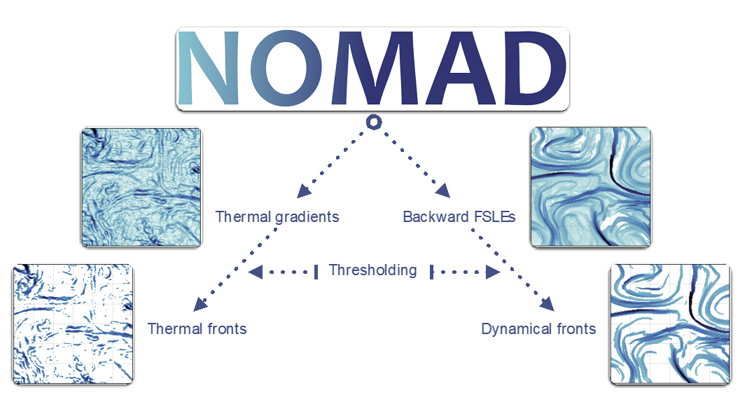
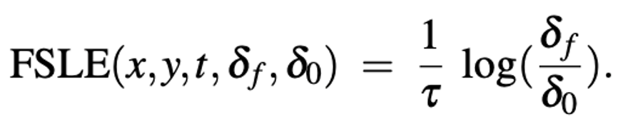
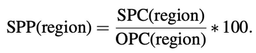
Thermal gradients We use the BOA (Belkin and O’Reilly, 2009), and more specifically Benjamin Galuardi’s pseudo-code written in R (available at: https://github.com/galuardi/boaR, accessed on May 19th, 2022) to compute thermal gradient magnitudes. We apply the BOA on daily satellite Sea Surface Temperatures (SST) from Multi-scale Ultra-high Resolution sea-surface temperature analysis (MUR SST, https://podaac.jpl.nasa.gov/dataset/MUR-JPL-L4-GLOB-v4.1, accessed on Jan 10th, 2023) (Chin et al., 2017), the resulting field is a thermal gradient expressed in °C/km. The resulting Southwestern Indian Ocean (SWIO) thermal gradient database covers latitudes between 5°S and 35°S and longitudes between 30°E to 80°E, and the Mediterranean Sea (MedSea) database covers latitudes between 30°N and 46°N and longitudes between -6°E to 37°E. The outputs for both geographical domains are produced daily from 2003 to 2020 and at the same spatial resolution of 1/100º which is about 1 km. Each daily thermal gradient map includes a flag variable indicating whether a given pixel is located on land (flag=2), or if it is "suitable" (flag=0) or "unsuitable" (flag=1) for thermal front analysis. Pixels are deemed "unsuitable" based on MUR SST standard deviation of the formal estimation error, which is considered to be a good estimate on MUR analysis uncertainty (Chin et al., 2017). When the MUR SST standard deviation of the estimation error is high, the thermal gradient field is smoothed out and possible front or eddy structures are obfuscated. We thus recommend applying the flag before any further analysis of the thermal gradient field. We set the MUR SST standard deviation of the estimation error threshold, i.e. threshold above which a pixel is deemed "unsuitable" for front analysis, at 0.0384°C. The choice of threshold is based on a preliminary comparison between MUR SST standard deviation and our thermal gradient dataset. Finite-Size Lyapunov Exponents In this work, backward-in-time FSLEs in the SWIO are computed from remotely-sensed Sea Surface Height (SSH) at 1/4° spatial resolution from Global Total Surface and 15m Current (CLS, 2018, COPERNICUS-GLOBCURRENT: https://resources.marine.copernicus.eu/product-detail/MULTIOBS_GLO_PHY_REP_015_004/INFORMATION, accessed on Jan 10th, 2023) from Altimetric absolute geostrophic velocities and Modeled Ekman Current Reprocessing (Rio et al., 2014}. In the MedSea, backward FSLEs are computed from daily absolute geostrophic surface currents derived from Sea Level Anomalies (SLA) at 1/8° spatial resolution from a SSALTO/DUACS multimission altimeter regional L4 product released in 2016 by AVISO+ and based on regional mean dynamic topography (Rio et al., 2014) (available at: https://data.marine.copernicus.eu/product/SEALEVEL_EUR_PHY_L4_MY_008_068/services, accessed on Feb 10th, 2023). Backward FSLEs were obtained following the algorithm described by Hernandez-Carrasco et al. (2011) Essentially, the algorithm computes backward FSLEs by integrating backward in time two neighbouring particle trajectories advected in a two-dimensional flow using a fourth order Runge-Kutta scheme with a bilinear interpolation in space and linear in time. The total period of integration is 90 days. The Runge Kutta time step was set at 6 hours to reduce numerical diffusion. As we are interested in simulating fluid particles, we computed trajectories of infinitesimal passive particles. The FSLE value at a given position and time (x, y, t) can be expressed as: delta_0 is the initial distance between a particle at (x, y, t) and its 4 closest neighbors. delta_0 corresponds to the spatial resolution of the FSLE grid, which is here 1/64° or approximately 1.56 km. delta_f is the final distance between particles, here it is set so that delta_f=10*delta_0. tau is the minimum time (among the 4 particle pairs) that it takes for the particles to reach the distance delta_f. FSLEs are thus expressed in day-1. Similarly to the thermal front dataset, the SWIO FSLE database covers latitudes between 5°S and 35°S and longitude between 30°E to 80°E, and the MedSea database covers latitudes between 30°N and 46°N and longitudes between -6°E to 37°E. Both geographical domains have a spatial resolution of 1/64° which is about 1.56 km, and the output is produced daily from 1994 to 2020. Each daily FSLE dataset includes a flag variable indicating whether pixels are located on land (flag=2), or if they are "suitable" (flag=0) or "unsuitable" (flag=1) for front analysis. Pixels are deemed "unsuitable" based on their FSLE value. Pixels whose FSLE value is 0 day-1 correspond to particles which have not reached the final distance delta_f after the integration time, i.e. after 90 days. Pixels whose FSLE value is above 900 day-1 correspond to beached particles. We thus recommend applying the flag before any further analysis of the FSLE field. Thresholds One of the advantages of using the BOA and backward FSLEs to detect fronts is that both output are continuous fields. Users can then determine the threshold above which thermal gradients or FSLE values belong to a meaningful front. Since different regions present different range of front intensity, that are somehow not-trivially linked to contrasting levels of Eddy-Kinetic Energy (Sudre et al., 2023), it is relevant to define region-specific thresholds. In order to adapt our database to users interested in the interaction between fronts and marine life we provide thresholds for the MedSea and the SWIO basins but also for each Longhurst's provinces (Longhurst, 1995 ; Longhurst, 2007) and Spalding's ecoregions (Spalding et al., 2007) falling into each geographical domain. For each regional and subregional dataset, we set the regional and subregional thresholds at the value of the 70th percentile computed over all the "suitable" pixels in the multidecadal database. Percentage of "suitable" pixels The percentage of "suitable" pixels in each region of interest (SPP) is given by: Where SPC is the number of "suitable" pixels in the region of interest and OPC is the total number of ocean pixels in the same region. Thresholds and SPP are provided for each region and subregion and as attributes in each netcdf file. For more detailed methodology and technical validation of NOMAD, please refer to: F. Sudre et al. NOMAD: the oceaN frOnt database for the Mediterranean seA and southwest inDian ocean. Submitted to Nature Sci Data (2023). References: Belkin, I. M. & O’Reilly, J. E. An algorithm for oceanic front detection in chlorophyll and sst satellite imagery. J. marine systems: journal Eur. Assoc. Mar. Sci. Tech. 78, 319–326, 10.1016/j.jmarsys.2008.11.018 (2009). Chin, T. M., Vazquez-Cuervo, J. & Armstrong, E. M. A multi-scale high-resolution analysis of global sea surface temperature. Remote. sensing environment 200, 154–169, 10.1016/j.rse.2017.07.029 (2017). Hernández-Carrasco, I., López, C., Hernández-García, E. & Turiel, A. How reliable are finite-size lyapunov exponents for the assessment of ocean dynamics? Ocean. modelling 36, 208–218, 10.1016/j.ocemod.2010.12.006 (2011). Longhurst, A., 1995. Seasonal cycles of pelagic production and consumption. Progress in Oceanography 36, 77–167. Longhurst, A., 2007. Ecological geography of the Sea. Academic Press, London. Rio, M.-H., Mulet, S. & Picot, N. Beyond goce for the ocean circulation estimate: Synergetic use of altimetry, gravimetry, and in situ data provides new insight into geostrophic and Ekman currents: Ocean circulation beyond goce. Geophys. research letters 41, 8918–8925, 10.1002/2014gl061773 (2014). Spalding, M. D. Fox, H. E. Allen, G. R. Davidson, N. Ferdana, Z. A. Finlayson, M. Halpern, B. S. Jorge, M. A. Lombana, A. Lourie, S. A., (2007). Marine Ecoregions of the World: A Bioregionalization of Coastal and Shelf Areas. Bioscience 2007, VOL 57; numb 7, pages 573-584. doi: 10.1641/B570707 Sudre, F. et al. Spatial and seasonal variability of horizontal temperature fronts in the Mozambique Channel for both epipelagic and mesopelagic realms. Front. Mar. Sci. 9, 10.3389/fmars.2022.1045136 (2023). |
| Constraints Contraintes |
|
| Spatial informations Informations géographiques |
|
Citation proposal Proposition de citation
Sudre Floriane , Ismael Hernández-Carrasco , Camille Mazoyer , Joel Sudre , Boris Dewitte , Véronique Garçon , Rossi Vincent (2023).NOMAD: the oceaN frOnt dataset for the Mediterranean seA and southwest inDian ocean.Ifremer
https://doi.org/10.12770/3ea321a1-d9d4-49e5-a592-605b80dec240
When using this dataset in a publication, also cite the related work(s) with:
Sudre, F., Hernández-Carrasco, I., Mazoyer, C. et al. An ocean front dataset for the Mediterranean sea and southwest Indian ocean. Sci Data 10, 730 (2023). https://doi.org/10.1038/s41597-023-02615-z
),POLYGON((79.875%20-34.875,79.875%20-5.125,30%20-5.125,30%20-34.875,79.875%20-34.875))))